

How to make predictions using Machine Learning in .NET and Python
How to make predictions using Machine Learning in .NET
Jacob Malling-Olesen is part of our Software Craftsman Program in which we ask our graduates and residents to write about different topics as part of their training to become Software Craftsmen.
In part 1 we saw that raw gathered data is rarely ready for use in ML. We then showed how to clean and transform the data to make it ready for Machine Learning.
Data Selection
It is now time to select the features to build the model upon. This is step 4 in the figure from part 1. In ML, features are the data values used for the prediction. The features being selected can be all available, but it can also be just one. This all depends on the performance of the trained model as this change depending on the selected features.
In the C# part this is where ML.NET starts to be used. First, a reader is specified where the header names are entered as the column list.
public static TextLoader CreateWeatherDataLoader(MLContext context)
        {
            TextLoader loader = context.Data.TextReader(new TextLoader.Arguments()
            {
                Separator = ";",
                HasHeader = false,
                Column = new[]
                {
                    new TextLoader.Column(nameof(_5HourInput.FutureTemperature), DataKind.R4, 0),
                    new TextLoader.Column(nameof(_5HourInput.Day_1), DataKind.R4, 1),
                    new TextLoader.Column(nameof(_5HourInput.Month_1), DataKind.R4, 2),
                    new TextLoader.Column(nameof(_5HourInput.Year_1), DataKind.R4, 3),
                    new TextLoader.Column(nameof(_5HourInput.Hour_1), DataKind.R4, 4),
                    new TextLoader.Column(nameof(_5HourInput.Temperature_1), DataKind.R4, 5),
      …
}
            });

            return loader;
  }
These names are then used when selecting which of these features to train the model with. After reading the data an EstimatorChain is created. This is basically a pipeline where features are selected using ML.NET transforms functions. In this pipeline it is also possible to do other kinds of transforms on the data, but since the data is already transformed, they are not used. Therefore, this pipeline is just a simple one where the feature to be predicted is selected and added to a column named “Label” while the features to predict is added to a column named “Features”.
var reader = MLDataReader.WeatherDataLoader.CreateWeatherDataLoader(mlContext);

            var trainData = reader.Read(new MultiFileSource(trainFilePath));

            var testData = reader.Read(new MultiFileSource(testFilePath));

            var dataProcessPipeline = mlContext.Transforms.CopyColumns("FutureTemperature", "Label")
                .Append(mlContext.Transforms.Concatenate("Features",
                nameof(_5HourInput.Temperature_1), nameof(_5HourInput.Humidity_1), nameof(_5HourInput.Dewpoint_1), nameof(_5HourInput.Barometer_1),
                nameof(_5HourInput.Windspeed_1), nameof(_5HourInput.Gustspeed_1), nameof(_5HourInput.Winddirection_1), nameof(_5HourInput.Rain_1),
In Python a library called Pandas is used. This is used for reading the data from disk and then in a list of strings it is specified which features to use while a single string specifies the value we predict.
trainDataFrame = pandas.read_csv(trainDataPath, sep=';').set_index(["Year_0", "Month_0", "Day_0", "Hour_0"])
testDataFrame = pandas.read_csv(testDataPath, sep=';').set_index(["Year_0", "Month_0", "Day_0", "Hour_0"])

predictors = ["Temperature_0", "Humidity_0", "Dewpoint_0", "Barometer_0", "Windspeed_0", "Gustspeed_0", "Winddirection_0", "Rain_0",
    "Temperature_1", "Humidity_1", "Dewpoint_1", "Barometer_1", "Windspeed_1", "Gustspeed_1", "Winddirection_1", "Rain_1",
    "Temperature_2", "Humidity_2", "Dewpoint_2", "Barometer_2", "Windspeed_2", "Gustspeed_2", "Winddirection_2", "Rain_2",
    "Temperature_3", "Humidity_3", "Dewpoint_3", "Barometer_3", "Windspeed_3", "Gustspeed_3", "Winddirection_3", "Rain_3",
    "Temperature_4", "Humidity_4", "Dewpoint_4", "Barometer_4", "Windspeed_4", "Gustspeed_4", "Winddirection_4", "Rain_4"]
labels = "FutureTemperature"

X = trainDataFrame[predictors]
y = trainDataFrame[labels]
Since scikit-learn needs us to specify which value is the label (“y”) and which value is the features (“X”) these are specified.
In both examples it is easy to remove or add the features that are used in the model without changing anywhere else in the code. So, there is not much difference on how to do this part in ML.NET or Python.
Model training
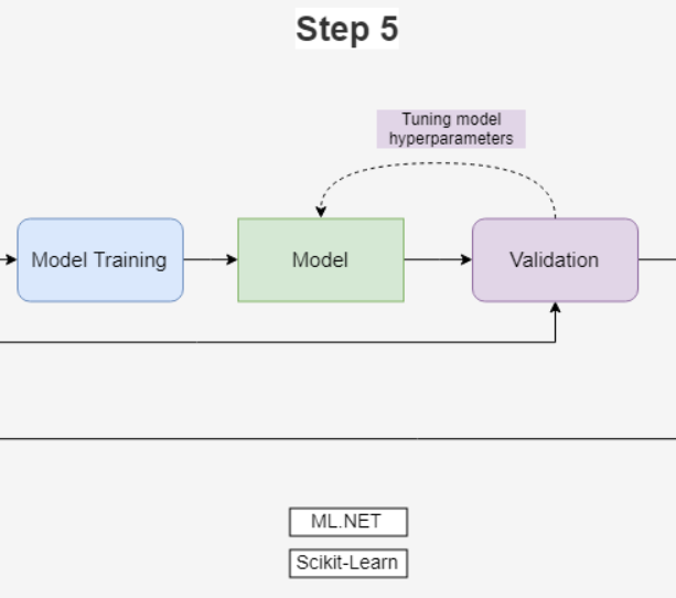
Now it is time to train the model as shown on figure 1. Since the goal is to predict a numerical value, a Regression training algorithm is chosen.
ML.NET contains some implementations of regression models. So first a trainer is selected and appended to the pipeline. When adding this it is possible to specify the featureColumn and the labelColumn (“Features” and “Label” by default) as well as some hyperparameters to tune the algorithm. Trying out the different algorithms with the right hyperparameters can be cumbersome only a few models with default parameters were tested before selecting the FastTreeTweedie model.
var dataProcessPipelineWithLearner = dataProcessPipeline.Append(mlContext.Regression.Trainers.FastTreeTweedie());

var model = dataProcessPipelineWithLearner.Fit(trainData);
The model is validated by testing how it performs on the data it was trained upon. This validation gives an average error of 0.72 degrees Celsius. Comparing this to general weather predictions it is not good, but not that bad either. The general way to determine if a model is “good enough” comes down to the problem it is trying to fix. For temperature prediction an average error of 0.72 might be fine while the same error for sensor data prediction could be unacceptable. Since this is just a small sample test, the model is deemed “good enough” to move on.
var validationData = model.Transform(trainData);
var validation = mlContext.Regression.Evaluate(validationData);
Console.WriteLine($"Validation: Mean Absolute Error {validation.L1}");
In Python this is a similar task since scikit-learn’s framework is used. Again, it is also possible to change hyperparameters and trainers. The LinearRegression trainer is the one that is chosen.
regressor = LinearRegression()
regressor.fit(X,y)
The validation of this model gives an average error of 0.38 degrees Celsius. This could seem like a decent score, so it is deemed “good enough”.
validation = regressor.predict(X)
print("Validation: Mean Absolute Error: %.2f" % mean_absolute_error(y, validation))
Model evaluation
The evaluation process resembles validation a lot, however there is one big difference. The data for the evaluation must never be part of the training. The way the model is evaluated is by performing the prediction on the test set. The predicted temperature is then compared to the correct temperature from the test set.
In ML.NET the Transform function is used to do the prediction. This transformed data is then given to a Regression Evaluation to get some evaluation metrics like Mean Absolute Error.
var evaluationData = model.Transform(testData);
var evaluation = mlContext.Regression.Evaluate(evaluationData);
Console.WriteLine($"Evaluation: Mean Absolute Error {evaluation.L1}");
The evaluation gives an average error of 0.52 degrees Celsius. Since it is not much worse than the validation average error it seems the model is not overfitting. Overfitting is when a model reaches close to perfect on the training data and then does not generalize well to new unseen input. I.e. the model only performs well in testing, not in production.
In Python the predict function is used on the features of the test data. This returns a list of temperature values that can be compared with the label of the test data. This comparison can be evaluation metrics like Mean Absolute Error.
Xtest = testDataFrame[predictors]
ytest = testDataFrame[labels]

evaluation = regressor.predict(Xtest)
print("Evaluation: Mean Absolute Error: %.2f" % mean_absolute_error(ytest, evaluation))
The evaluation gives an average error of 0.36 degrees Celsius. Again, the value is not worse than the validation average error.
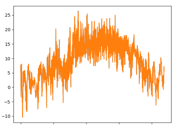
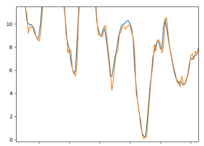
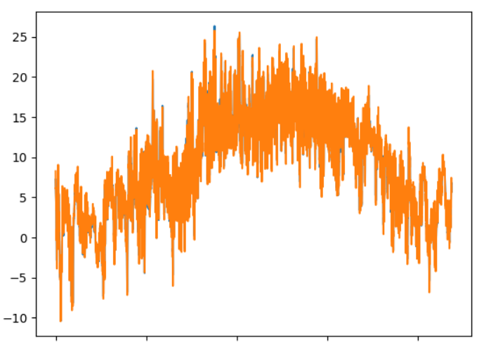
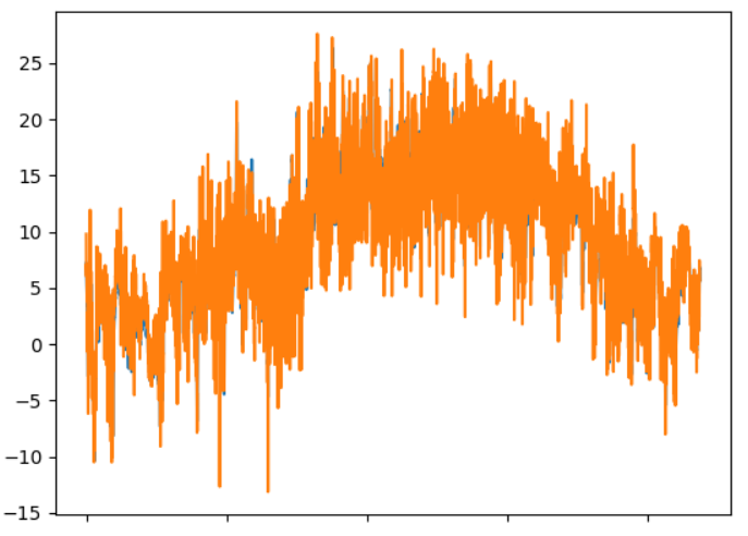
Instead of relying on raw data values like Mean Absolute Error we can also plot our true data and our predicted data next to each other to visualize the comparison. In Python this can be done using PyPlot. Adding the true evaluation values (blue) and the predicted (orange) to the same plot it can be hard to see the difference, so we need to zoom in:
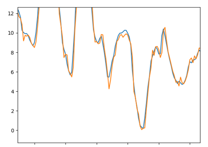
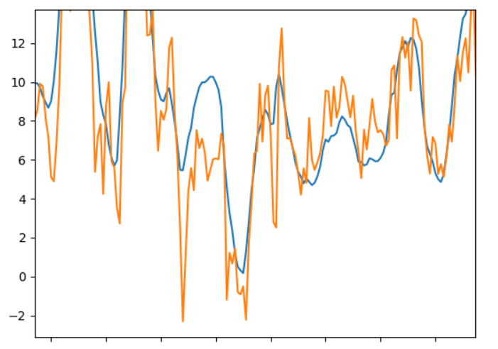
Here it is possible to see some difference. Generally, the predictions seem to follow the true values. However, at some points the values have the same increase and decrease but are shifted a little along the x-axis. This means the prediction on the given time date would be a little off resulting in more error in the prediction when comparing it to the true value.
A problem with these evaluations is that for weather prediction just looking ahead 1 hour doesn’t seem that interesting. It would be much more interesting to be able to predict multiple hours ahead using its own temperature predictions as input and see how well the models perform on this task. So, implementing a specific evaluation function to evaluate the performance each hour up to five hours ahead seems like a good idea. Since the models uses multiple parameters, all other features but the temperatures are faked in the evaluation as they would otherwise have to be predicted as well by other models or more sophisticated models able to return multiple values.
In ML.NET this is a function that takes a PredictionFunction generated from the trained model and then a data file containing the test set. Then going through five timeseries datapoints at a time it calculates the FutureTemperature and uses this value as the temperature value in the next datapoint.
public void Evaluate(PredictionFunction<_5HourInput, PredictionValue> predictor, string testFilePath)
        {
            var input = new TimeseriesDataAccessor().Read(testFilePath);
            var testData = timeseriesTo5Hour(input);

            var totalError = 0f;
            var totalError2 = 0f;
            var totalError3 = 0f;
            var totalError4 = 0f;
            var totalError5 = 0f;

            for (int i = 0; i < testData.Count() - 5; i++)
            {
                var prediction = predictor.Predict(testData.ElementAt(i));
                var totalError += MathF.Abs(prediction.FutureTemperature - testData.ElementAt(i).FutureTemperature);
…
The results of this evaluation:
| Hours in future | 1 | 2 | 3 | 4 | 5 |
| Average error | 0.52 | 1.29 | 2.02 | 2.7 | 3.3 |
This table shows that the error quickly increases. Even though it initially looked okay with half a degree error it quickly accumulates to more than three degrees error on average after five hours.
In Python this looks just the same. Using the model and a testFilePath as input the function does the calculations in a for-loop.
def Evaluate(self, model, testFilePath):
  testDataFrame = pandas.read_csv(testFilePath, sep=';').set_index(["Year_0", "Month_0", "Day_0", "Hour_0"])
  predictors = ["Temperature_0", "Humidity_0", "Dewpoint_0", "Barometer_0", "Windspeed_0", "Gustspeed_0", "Winddirection_0", "Rain_0",
      "Temperature_1", "Humidity_1", "Dewpoint_1", "Barometer_1", "Windspeed_1", "Gustspeed_1", "Winddirection_1", "Rain_1",
      "Temperature_2", "Humidity_2", "Dewpoint_2", "Barometer_2", "Windspeed_2", "Gustspeed_2", "Winddirection_2", "Rain_2",
      "Temperature_3", "Humidity_3", "Dewpoint_3", "Barometer_3", "Windspeed_3", "Gustspeed_3", "Winddirection_3", "Rain_3",
      "Temperature_4", "Humidity_4", "Dewpoint_4", "Barometer_4", "Windspeed_4", "Gustspeed_4", "Winddirection_4", "Rain_4"]
  labels = "FutureTemperature"

  Xtest = testDataFrame[predictors]
  ytest = testDataFrame[labels]

  totalError = 0
  totalError2 = 0
  totalError3 = 0
  totalError4 = 0
  totalError5 = 0

  for i in range(0,len(Xtest)-5):
    prediction = model.predict([Xtest.iloc[i]])
    totalError += abs(prediction[0] - ytest.iloc[i])
The results of this evaluation:
| Hours in future | 1 | 2 | 3 | 4 | 5 |
| Average error | 0.36 | 0.89 | 1.49 | 2.29 | 3.25 |
The table again shows the tendency of the increasing error the further into the future the prediction goes.
Plotting these data in a similar fashion as above:
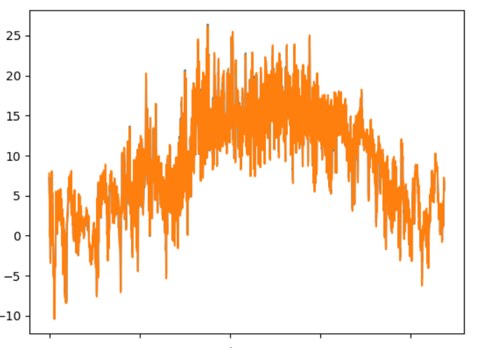
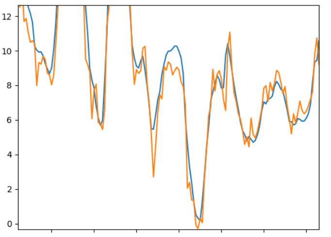

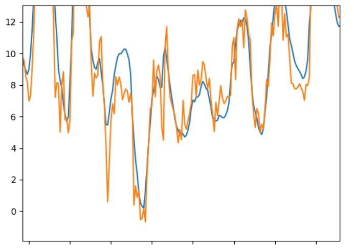
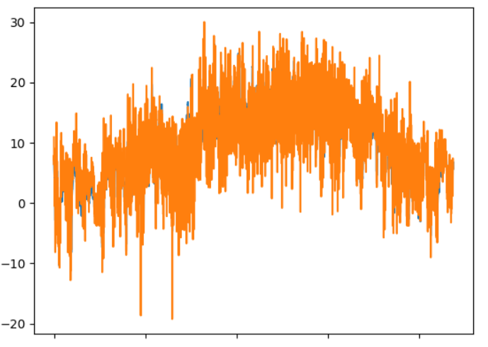
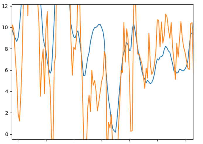
These plots show the same tendency as the tables. And in the fifth plot there is not much coherence between the blue and orange lines.
These evaluations show how important it is to fit the evaluations to the task that should be completed. Using the standard evaluation, it could be tempting to release the model, as an average error of half a degree Celsius in temperature predictions does not seem that bad. This evaluation would also deem the model not “good enough”. Therefore, going back to step 5 and selecting another training algorithm or even back to step 4 and select other data features would be the next step in this process. Should it happen that testing all kinds of different training algorithms and data features still doesn’t provide a model that performs “good enough” gathering more data or different data could also be a way to tackle this.
All in all, there is not much difference in the coding style of ML.NET and Python with Pandas and scikit-learn. The frameworks also work similarly and uses many of the same terminologies. One of the biggest differences is the number of training algorithms in the two frameworks where scikit-learn takes the lead. However, ML.NET is being worked on extensively with new updates coming monthly. So, the choice of which framework to select comes down to which language best fits the system that should incorporate machine learning as well as other organizational demands such as performance and maintenance.
About the author
Jacob Malling-Olesen is a computer scientist specialised in Machine Learning. He is now a graduate attending our Software Craftsman Program. We encourage our graduates to write about the things they learn as we believe that software craftsmanship is based on continuous learning.
Do you want us to help you with Machine Learning projects?
Morten Hoffmann
CEO
T: (+45) 3095 6416 E: mhs@strongminds.dk